Visualizing stochastic processes and martingales
Visualizing fields generated by a stochastic process
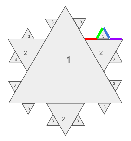
The fractal triangles shown below can help us visualize a simple stochastic process \(\{x_1, x_2, x_3\}\) (corresponding to times \(t_1, t_2, t_3\)).

Before time \(t_1\), the value taken by \(x_1\) is not yet determined; at \(t_1\) and later, the value taken by \(x_1\) is determined, and we say that we have measured \(x_1\). And similarly for \(x_2\) and \(x_3\).
We can think of each random variable \(x_i\) as a 3-sided dice (in the case of \(x_1\)) or a 4-sided dice (in the case of \(x_2\) and \(x_3\)). So for example, let’s say we roll dice 1 and get the right-face, and then we roll dice 2 and get the up-face. And now we are poised to roll dice 3 (but have not yet done it), and we know that the dice 3 roll could have 4 possible results. The image of \(x_3\) contains 4 possible values, corresponding to the four colors (red, green, blue, purple); the probability of measuring each value is given by the measure of its corresponding colored segment. This situation is illustrated in the figure.
Let \(\Omega\) be the set of all possible outcomes for rolling the three dice. Then we can think of \(\Omega\) as all the points in the border of the figure (i.e., all the points that are on the external border of the multi-fractal-triangle object). Let \(W\) = the event that consists of the four colored segments in the figure above. \(W\) is a subset of \(\Omega\); we call it the event {“Dice 1 rolled right-face” and “dice 2 rolled up-face”}. It is 1 of 12 events of this type because there are 12 ways that dice 1 and dice 2 could have turned out.
These 12 events form a partition \(P\) of \(\Omega\) that generates the field \(F_2\), which is also called the field generated by \(x_1\) and \(x_2\).
Visualizing a conditional expectation
The conditional expectation \(E[x_3 \mid x_1,x_2]\) is the expected value of \(x_3\) given the measurement results for \(x_1\) and \(x_2\). Unlike a regular expectation (i.e., unlike an expectation that is NOT conditional), it is not a real number. Instead, the conditional expectation is a random variable that maps any outcome in \(\Omega\) to a real number.
So in this example, if the outcome \(\omega \in \Omega\) is in the event \(W\) (the four colored segments), meaning that \(W\) is true, then \(\omega\) is mapped by the random variable \(E[x_3 \mid x_1,x_2]\) to the average of \(x_3\) over the event \(W\). Any other \(\omega \in W\) is mapped to the same real number. We can think of this as: take any outcome \(\omega \in \Omega\), find the event \(p \in P\) that contains it (i.e., the event in \(P\) with the \(x_1\) and \(x_2\) values that are consistent with \(\omega\)), and average \(x_3\) over the event \(p\) to produce the answer. (Recall that \(P\) is the partition that generates the field \(F_2\), where \(F_2\) is the field generated by \(x_1\) and \(x_2\). So each \(p \in P\) is an event that contains all possible \(\omega\) with consistent values of \(x_1\) and \(x_2\).) Intuitively, it’s as if \(\omega\) could hide from us the information regarding which \(x_3\) it corresponds to, so that all we know is which \(p \in P\) contains that \(\omega\), so that our best estimate for \(x_3\) is to take its average value over that event \(p\).
We want to discuss martingales, so let’s also think about the meaning of \(x_2\). \(x_2\) is a random variable that maps an outcome that is anywhere on the outline of the figure (\(\Omega\)) to one of the values in the image of \(x_2\), with the probability of each possible value given by the total measure of the corresponding segments that map to that value.
Visualizing a martingale
So here is how we think about a martingale-like behavior where
\[E[x_3 \mid x_1,x_2]=x_2.\]For any outcome \(\omega \in \Omega\), find the event \(p \in P\) that contains \(\omega\). Then \(x_2\) takes on a single fixed value \(x_2(p)\) over the entire event \(p\); this is the right hand side of the martingale condition. And we require the left hand side of the martingale condition, the average of \(x_3\) over the event \(p\), to be equal to \(x_2(p)\).

Looking back at the fractal triangles, taking the event \(W\) (the four colored segments) as an example, \(x_2\) takes on a single value \(x_2(W)\) over the entire event \(W\), so we require the average of \(x_3\) over the four colored segments to be equal to that value \(x_2(W)\).
This is the meaning of the martingale condition.